The winning solution for InnoCentive Challenge
“Calculation of the Intrinsic (Maximum) Birefringence of Molecules”
In brief the challenge was formulated as following: predict experimental birefringence (Dn, with 10% error) for pure liquid crystal substances, at the wavelength of 550 nm, using only their molecular structure as input.
It is not possible to apply some form of Lorentz-Lorenz (LL) equation to a single molecule to obtain birefringence value (Dn) for a simple reason that the polarizability (a) is a molecular property, but refraction coefficients (n) and Dn are the properties of the condensed phase. And this is explicitly expressed in the LL equation by the term N (number density, a number of molecules per unit volume).
Therefore, in order to apply the LL equation certain assumptions about the phase need to be taken. E.g. in a crystal we know that all the molecules arranged in a certain orientation in relation to each other, and fixed. So, the LL equation can produce adequate n for certain crystals.
In the proposed solution the assumption was made that the liquid crystals form nematic phase, meaning that they generally keep their orientation along the director (x axis), but their positions are not fixed and they are able to rotate about their internal x axis:


The first figure is from ref. [1]; the second one is the representation of the nematic phase, as used in the challenge solution.
Brief Summary
Total 270 variations of five selected methods were tested for the calculation of birefringences (Dn). None of them were capable of direct reproduction of experimental values with satisfactory accuracy. However, many of these methods produced results, which excellently correlate with the experiment (r>0.95). Three best linear correlation functions were selected as a solution for the challenge. One method uses only properly optimized molecular structure (mol2 file); other two require additional calculation of molecular polarizabilities (a) using time dependent Hartree-Fock (TDHF) method as realized in Firefly (former PC GAMESS) and GAMESS programs. Application of these correlation functions allows for calculation of Dn with error less than 10% for nematic or smectic liquid crystals for diverse molecular structures.
The selected methods are nicknamed “Vuks”, “Direct”, and “Order”. The correlation charts between calculated and experimental Dn are shown in Fig. 1, and the test results are in Table 1.
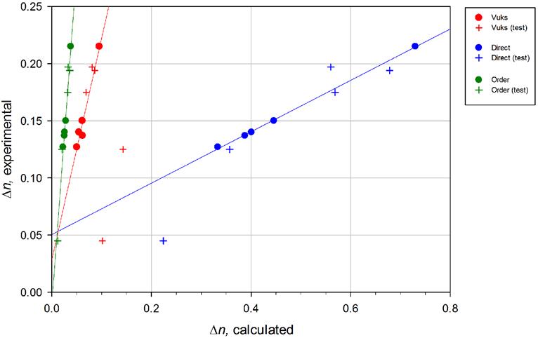
Figure 1. Correlation graphs for the three methods of the calculation. Circles — data points of five substances used for regression analysis. Crosses — data points for substances used to test the calculation method.
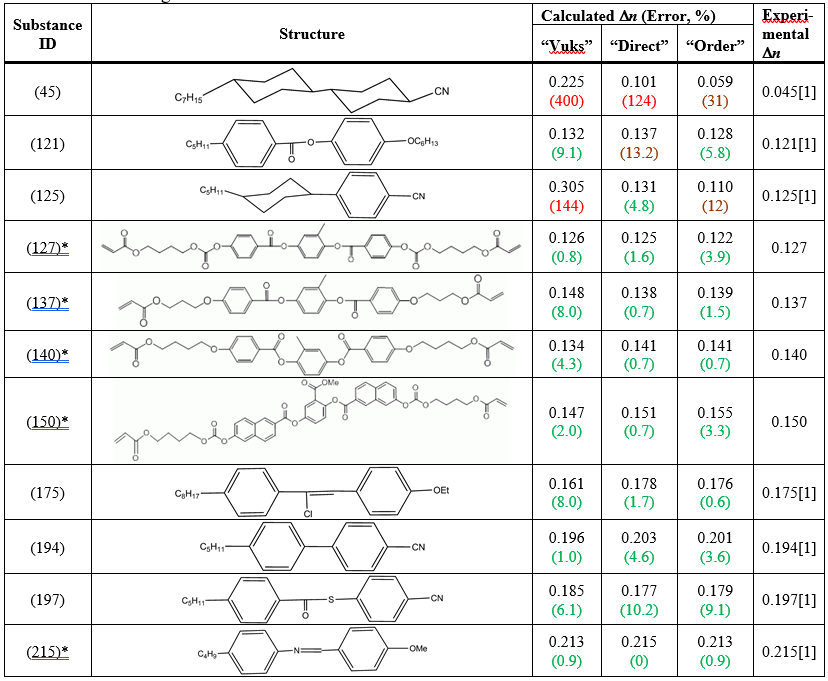
Table 1. The results of calculations for the three selected methods.
Toolbox required
- General purpose molecular modeling program, which allows to build the molecule, read and write mol2 files, and align the molecule along x and y coordinate axes.
- Open Babel to prepare the input files and extract optimized structures.
- Ab initio computational chemistry program: Firefly or GAMESS.
- The molecular alignment utility (mol2align, supplied by XR Pharmaceuticals).
- The birefringence calculator dn_corr (supplied by XR Pharmaceuticals).
Steps to calculate birefringence
1. Create the structure of interest in your molecular modeling package and check that it has “reasonable” 3D structure (no exaggerated angles or bonds). If it doesn’t look right, perform a “cheap” structure optimization (e.g. by using molecular mechanics or semi-empirical PM3 method available in most modeling software).
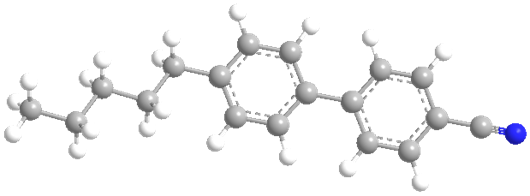
As an example I will use structure (194) from Table 1:
Distorted (for whatever cause) structure:

“Reasonable” structure (if the substance has biphenyl fragment like the one below, make sure that the starting dihedral angle between the two rings is non-zero, otherwise the optimization may end up in incorrect planar configuration):
By convention, the resulted file is saved as 194.mol2 (substance ID is used as the file name).
2. Prepare the input for fine structure optimization using RHF method, 6-311+G(d,p) basis set [2] in Firefly. This is done by Babel with the following command:
babel.exe -imol2 194.mol2 -ogamin 194.inp -xf header_opt.inp
Where “header_opt.inp” is the header file for the RHF method above.
3. Run the structure optimization with Firefly using the input file (194.inp) produced in step 2. For the sample compounds in Table 1 the time of calculation was about 6–8 hr. (in 2013) on an Intel Core i7 processor with 4 cores.
4. Extract the optimized structure into mol2 file from Firefly output using Babel:
babel.exe -igamout Firefly_output_file -omol2 194.mol2
5. Very important! Open the optimized mol2 file from step 4 in your modeling program, and align the longest direction of the molecule with the x axis, and “widest” direction with the y axis, so that the molecule will be oriented approximately along the principal axes of the tensor of molecular polarizability, like on the following illustrations taken from [1]:

Save mol2 file, overwriting the old one.
Preferred method is to use the mol2align program using the command
mol2align.exe xxx.mol2
producing xxx_aligned.mol2 file, which needs to be checked e.g. in Chimera package. The properly aligned molecule will have overall molecular plane lying in xy-plane, the longest molecular axis aligned with x-axis, and molecular center of mass at the origin.
6. After step 5 you already can do the Dn calculation by “Vuks” method using the following command:
dn_corr.exe 194.mol2
The result will be written to “194.mol2.out” file (more on the result format below).
7. To use “Direct” and “Order” methods it is necessary to calculate molecular polarizabilities at 550 nm using TDHF method in Firefly. So, in this step you will prepare the input file for Firefly using optimized and aligned mol2 file from step 5:
babel.exe -imol2 194.mol2 -ogamin 194.inp -xf header_tdhf.inp
Where “header_tdhf.inp” is the header for polarizability calculation at 0 and 550 nm.
8. Run Firefly with the input file produced in step 7. Depending on the structure, full calculation in 2013 would take 2–4 hrs on Intel Core i7, 4 cores run in parallel. The following strings from the Firefly output must be copy-pasted into 194.out for further calculations:
*****************************************************************
 CALCULATION FOR A FREQUENCY OF    2.25425 EV  (   0.08284 A.U.)
                  WAVELENGTH OF    550.00 NM
 *****************************************************************
 ......................................................................
 ALPHA AT    0.08284 A.U.
 ......................................................................
 ..... INITIATING DIIS PROCEDURE .....
 MAXIMUM RESPONSE VECTOR ERROR= 1.233805E+00
 MAXIMUM RESPONSE VECTOR ERROR= 1.673674E-01
ALPHA XX =           357.96100098340820 UA CONV. TO 4.70E-06 IN 17 ITER.
    ALPHA YX =              14.22455326214941
    ALPHA ZX =              -7.30887739164954
 ..... INITIATING DIIS PROCEDURE .....
 MAXIMUM RESPONSE VECTOR ERROR= 3.708951E-01
 MAXIMUM RESPONSE VECTOR ERROR= 7.088355E-06
ALPHA YY =          181.54755787106600 UA CONV. TO 6.47E-06 IN 16 ITER.
    ALPHA XY =              14.22453535016288
    ALPHA ZY =               6.52190907992419
 ..... INITIATING DIIS PROCEDURE .....
 MAXIMUM RESPONSE VECTOR ERROR= 7.319860E-02
 MAXIMUM RESPONSE VECTOR ERROR= 4.290535E-02
 ALPHA ZZ =         106.71731105211180 UA CONV. TO 9.86E-06 IN 14 ITER.
    ALPHA XZ =              -7.30887464741015
    ALPHA YZ =               6.52190977584003
  ISOTROPIC AVERAGE ALPHA =             215.40862330219530 A.U.
It is possible to use other quantum chemical programs (Gaussian, MOPAC etc.), the results of polarizability calculation must be extracted and put in the “.out” file manually according to the following format (blanks are important!):
ALPHA AT 0.08284 A.U.
ALPHA XX = 357.96100098340820
ALPHA YX = 14.22455326214941
ALPHA ZX = -7.30887739164954
ALPHA YY = 181.54755787106600
ALPHA XY = 14.22453535016288
ALPHA ZY = 6.52190907992419
ALPHA ZZ = 106.71731105211180
ALPHA XZ = -7.30887464741015
ALPHA YZ = 6.52190977584003
9. Calculate birefringence by all three methods using mol2 file from step 5 and .out file from step 8:
dn_corr.exe 194.mol2 194.out
The calculation produces short output file “194.mol2.out”, containing the following information for the three methods (comments are in red):
-----------------------------------------------------
Birefringence calculation for: 194.mol2
S parameter:  0.910                               Used for “Order” method
D parameter:  0.000                              Used for “Order” method
Number density (N):  2.414                       See the technical details below
Contribution of ny to no:  0.900                 See the technical details below
Contribution of nz to no:  0.100
------------------------------------------------------
Polarization tensor from structure (nm^3):       Derived from mol2 file
 0.0271 0.0000 0.0000
 0.0000 0.0245 0.0000
 0.0000 0.0000 0.0245
###
Vuks calculations
NX:  2.1708                                      x component of n
NY:  2.0845                                      y component of n
NZ:  2.0845                                      z component of n
N_AVERAGE:  2.1132                               <n>
NO:  2.0845                                      n┴
NE:  2.1708                                      n||
DN:  0.0863                                      Dn calculated

Predicted birefringence from mol2 structure:  0.196   Final predicted Dn based on the correlation, your main result
-------------------------------------------------------
TDHF calculation at  0.08284 a.u. (550.0 nm)
Polarization tensor from TDHF (nm^3):            Derived from TDHF calc.
 0.0530  0.0021 -0.0011
 0.0021  0.0269  0.0010
-0.0011  0.0010  0.0158
###
DIRECT calculations
NX:  2.1146
NY:  1.4564
NZ:  1.2534
N_AVERAGE:  1.6082
NO:  1.4361
NE:  2.1146
DN:  0.6784
DN_ERROR:  0.0 %

Predicted birefringence from DIRECT TDHF:  0.203
###
ORDER calculations
NX:  2.1146
NY:  1.4564
NZ:  1.2534
N_AVERAGE:  1.6082
NO:  1.0743
NE:  1.1104
DN:  0.0361
DN_ERROR:  0.0 %

Predicted birefringence from ORDER TDHF:  0.201
Technical details
In the course of algorithm development general approach was to:
1. Obtain molecular polarizabilities (a) for a given molecule;
2. Calculate parallel and perpendicular components of the refractive index (n|| and n┴ correspondingly).
The computation methods selected for the final solution will be described below.
Molecular polarizabilities(a)
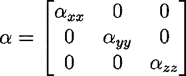
Two procedures were tested for the calculation of the molecular polarizability tensor
1. The bond increment procedure described in [3, 4], with slight modifications.
Each chemical bond in the molecule is assumed to contribute certain increment to the total molecular polarizability. The increments, which are currently in the program database, are listed in Table 2. This increment depends on the bond’s orientation in relation to the main directions of the polarizability tensor (hence the importance of the step 5 of molecule alignment above), and the final increments were calculated as following:
For each bond i:
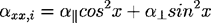

Where (x,y,z) are the angles formed by the bond i and axes x, y, z correspondingly, and a||, a┴ are the bond values from Table 2.
The final molecular polarizability is the sum of all bonds’ increments:

This calculation requires only properly optimized and aligned molecular structure, but is limited only to the types of bonds listed in Table 2 (if necessary, it could be extended), and very sensitive to the orientation of the molecule and its conformation.

The last fact could be the main reason why it didn’t work for conformationally labile compounds, like cyclohexane derivatives (45) and (125) from Table 1. For rigid molecules made of aromatic rings conjugated through C=C bonds and heteroatoms (O,S,N) this method works surprisingly well.
2. Calculation of molecular polarizabilities using time-dependent Hartree-Fock method at 550 nm.
This method is implemented in high quality quantum chemical packages Firefly and GAMESS, and described in [7, 8]. It allows for calculation of a at a given experimental wavelength (550 nm), and does not appear to be that sensitive to the molecule orientation. The input for this method is the same molecule as for the previous one (see calculation steps above).
The basis set was adopted from ref. [2], where it had been used to calculate non-linear optical properties of azulenes. As long as it produced acceptable results, I did not investigate any further.
So far most the most important part in practical predictions of Dn is not the accuracy of polarizability, but the consistency of the procedures. By the latter I mean that all computation procedures must be performed in exactly the same manner. No matter how accurate are polarizabilities, the uncertainty of the phase structure will nullify that. Yet, as mentioned before, none of the methods used are able to reproduce experimental Dn directly. However, many methods produce Dn in excellent correlation with the observed values. The equation below is of the utmost importance for the success of birefringence prediction.
Dnexperimental = aDncalculated + b
Where a and b are the linear regression coefficients. For the time being these are just phenomenological coefficients resulting from the regression analysis. They cover any uncertainty in the calculations of polarizabilities, and lack of understanding of molecules interaction in the mesophase.
If one wishes to pursue fundamental investigation of the mesophase optics then, probably, robust DFT calculations will help to get rid of the first uncertainty (polarizabilities will be very accurate). If the only need is to practically predict the birefringence, then there’s no reason to use more costly methods.
In any case, the regression coefficients above must be found separately for any method used. And, to be on the safe side, even for the same method used by different quantum chemistry package (e.g. Gaussian).
Refractive indices (n|| and n┴)
1. “Direct” calculation.
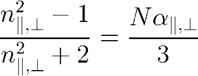
“Direct” method uses the Lorentz-Lorenz equation [1, 9, 10] to calculate the components of refractive indices:

Where ni are refractive indices along x, y, or z axes, and N is the number density (number of absorbing molecules). As long as the main unit of polarizability in calculations is nm3, N is measured as the number of absorbing molecules per nm3.
Two ways of calculating N were tried: N = 1/molecular volume (nm3), and N calculated from the molecular mass assuming that density of most liquid crystals is around 1 g/ml: N = 602/Mr. The last formula demonstrated better results , so it was used throughout to determine N.
Three calculated refractive indices were reduced to the main two, n|| and n┴ by the following approach:
n|| = nx (5)

Where fn,y is the fraction contributed by ny, and 1- fn,y is the fraction contributed by nz. The values of fn,y in the range from 0.1 to 0.9 were tested for all calculation methods, but they had little or no influence on the final correlation functions. In simple terms, the exact contribution of ny or nz to n┴ is not important for Dn.
2. “Vuks” calculation.
It uses a variation of Lorentz-Lorenz equation first suggested by Vuks [3, 9-11], assuming that the internal field in the condensed phase is isotropic:

Here ni2+2 is replaced by an average of squares of all n components. Therefore, in order to find ni from Vuks equation it is necessary to solve a system of three equations.
All other details for calculation of N, n|| and n┴ are the same.
3. “Order” calculation.
The method is adopted from [1], pg. 116 onwards. A modified form of Lorentz-Lorenz equation is used:
For this equation a|| and a┴ are calculated using liquid crystals order parameters S and D:


The order parameters S and D reflect the anisotropy of liquid crystals, decreasing with the temperature, and finally zeroing out at the clearing point. For the present solution a consensus value of S = 0.91at 25ºC has been chosen [12], while D was ignored and left out to be zero [1].
The calculations for N were done as in “Direct” method.
Regression analysis
As it has been noted in the summary, none of the methods was capable of reproducing the experimental values of birefringence with acceptable accuracy. However, when the experimental Dn were plotted against calculated ones, many methods produced very clear linear correlation plots (Fig. 1) with regression coefficient r>0.95.
In the linear regression analysis, the data of only five compounds from Table 1 were included. The other compounds were used to test the final selected algorithms.
Below is the final brief of the three methods selected for the solution is given, together with corresponding linear regression equations.
1. “Vuks” method (adopted from [3])
a: calculated from bond increments;
n: calculated according to Vuks [3, 11].
Regression equation: Dnexperimental = 1.9392Dncalculated + 0.0282; r = 0.983
Comments: Requires only properly optimized structure (mol2 file), works fine for rigid molecules (error <10%, see Table 1); doesn’t work for flexible molecules like cyclohexane derivatives (error>100%); sensitive to molecule’s orientation; suitable only for limited set of chemical bonds (Table 2).
2. “Direct” method
a: calculated from TDHF;
n: calculated according to the LL equation.
Regression equation: Dnexperimental = 0.2249Dncalculated + 0.0505; r = 0.999
Comments: Requires properly optimized structure, and the output from TDHF calculation; works well for all but very flexible molecules like dicyclohexane derivatives (typical error <10%, see Table 1).
3. “Order” method
a: calculated from TDHF;
n: calculated using the order parameter S.
Regression equation: Dnexperimental = 5.8643Dncalculated -0.0112; r = 0.994
Comments: Could be recommended as the best of all three methods. Requires properly optimized structure, and the output from TDHF calculation; worked for all tested compounds (error <10%, with one exception, when error is 12%, see Table 1). The large error for compound (45) of 31% is due to small experimental value of Dn (0.045), otherwise the absolute error in this case is comparable to other substances.
References
1. Demus, D., Physical properties of liquid crystals1999, Weinheim ; New York: Wiley-VCH. 503 pp.
2. Karakas, A., et al., Ab-initio calculations on static and dynamic third-order optical nonlinearity of azo-azulenes. Photonics Letters of Poland, 2012. 4(1): p. 17-19.
3. De Jong, S. Groeneweg, and V. Van Voorst, Calculation of the Refractive Indices of Molecular Crystals. J. Appl. Cryst., 1991. 24: p. 171-174.
4. Subramhanyam, H., C. Prabha, and D. Krishnamurti, Optical Anisotropy of Nematic Compounds. Mol. Cryst. Liq. Cryst., 1974. 28: p. 201-215.
5. Lippincott, E. and J. Stutman, Polarizabilities from d-Function Potentials. J. Phys. Chem., 1964. 68(10): p. 2926-2940.
6. Smith, R. and E. Mortensen, Bond and Molecular Polarizability Tensors. II. Discussion of Values of Polarizability Parameters for Some Single Bond Involving Carbon. J. Chem. Phys., 1960. 32(2): p. 508-511.
7. Shelton, D. and J. Rice, Measurements and Calculations of the Hyperpolarizabilities of Atoms and Small Molecules in the Gas Phase. Chem. Rev., 1994. 94: p. 3-29.
8. Korambath, P. and H. Kurtz, Frequency-Dependent Polarizabilities and Hyperpolarizabilities of Polyenes, in ACS Symposium Series 628. Nonlinear Optical Materials. Theory and Modeling, S. Karna and A. Yeates, Editors. 1996, ACS: Washington DC. p. 133-144.
9. Li, J. and S.-T. Wu, Self-consistency of Vuks equations for liquid-crystal refractive indices. J. Appl. Phys., 2004. 96(11): p. 6253-6258.
10. Kumar, A., Calculation of Optical Parameters of Liquid Crystals. Acta Physica Polonica A, 2007. 112(6): p. 1213-1221.
11. Vuks, M., Determination of optical anisotrophy of aromatic molecules from crystal birefringences. Optika i Spektroskopiya (Optics and Spectroscopy, in Russian), 1966. 20(4): p. 644-651.
12. Hauser, A., et al., Order Parameter and Molecular Polarizabilities of Liquid Crystals with Nematic and Smectic Phases. Mol. Cryst. Liq. Cryst., 1983. 91: p. 97-113.